The roots of this blog post were planted in a post I published very recently regarding the Audio First Fidelia. I began, while drafting that post, to explain some of the techniques and technology used to carry out acoustic measurements of speakers, the Klippel NFS (Nearfield Scanner) in particular, but it soon became obvious that the NFS deserved a post of its own. The rhetorical question that sent me off on an explanation of speaker measuring was, “ What’s a Klippel NFS and what does it do?” Hopefully the following few paragraphs will provide some answers.

Measuring the acoustic performance of a speaker isn’t as simple as it might appear. You can of course put a calibrated measurement microphone in front of a speaker and capture some data as the speaker is fed with a known signal. However, any acoustic reflection of the speaker output from the floor, ceiling or walls (or anything else in the vicinity) that also makes its way to the microphone will get mixed in with the direct sound from the speaker. Disentangling the resulting mess is all but impossible, so you can never really know what in the data is the speaker, and what is the “room”. Traditionally, there’s been two approaches that offer a fix to this.

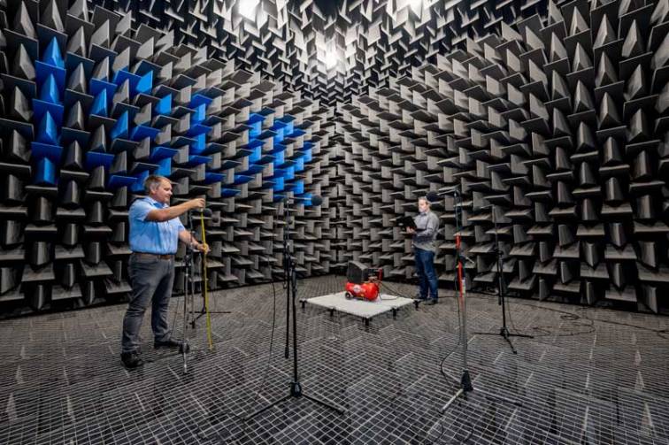
Firstly, there are anechoic (without echos) chambers designed to offer a space that’s completely free of reflections. The problem with anechoic chambers is that in order to fully absorb low frequency sound energy they have to be huge. This is because low frequency sound has a very long wavelength (17m at 20Hz). And being huge equates to being very expensive. The UK’s largest commercially available anechoic chamber is at Southampton University. It is 9.15m x 9.15m x 7.32m internally (without its foam wedges) but provides truly anechoic performance only down to about 80Hz.

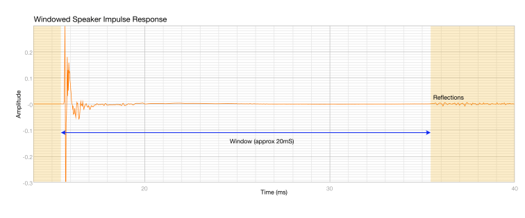
The second measurement fix is to use “windowed” data. If the measurement signal sent to the test speaker is an impulse (or a signal from which the impulse response can be mathematically derived) it is possible to capture it and then mute the measurement (shut the window) just before the first reflection arrives; any reflected acoustic energy is then not included in the data. This kind of technique has substantially replaced the use of anechoic chambers, but it is still flawed.

The flaw arises from the length of the time window before the first reflection arrives; the shorter that window the higher will be the cut-off frequency in terms of measurement accuracy. For example, if the window before the first reflection arrives is, say 10mS long, the measurement can only be accurate above 100Hz (1/10mS)*. This is because, to be accurately analysed, a full cycle of periodic data must be included in the window. A full cycle at 100Hz takes 10mS so if  the measurement window were to shut at, say 7mS, a 100Hz signal can’t be accurately measured because it simply won’t fit in the window. Now, the speed of sound is 343m/S, so it travels 3.43m in 10mS, which means that for a 10mS measurement window, the nearest reflective surface must be at least 3.43 metres further away from the measurement microphone than the speaker. Perhaps you can see where I’m going with this? That is, while you don’t need the foam wedges of an anechoic chamber for windowed measurements, you still need a pretty big (and very quiet) space. Finally, you may have realised that the contents of our data window is simply the impulse response of the speaker, and while you can tell a few things about a speaker from examining its impulse response, you need some computational power to carry out a Fourier transform in order to generate frequency domain data (the speaker frequency response curve that we’re probably all familiar with). So, while windowed measurement techniques are definitely an advance on anechoic based techniques (mostly because they are more practical), they are still flawed.

Those few paragraphs of background bring me to answering the original question – What’s a Klippel NFS? To start with a little history, Prof. Wolfgang Klippel is a speaker, acoustics and psycho-acoustics specialist who in 1997 founded a company dedicated to developing innovative acoustic analysis techniques. From modest beginnings, Klippel GmbH has grown to become probably the world leader in innovative speaker test and measurement technologies, and one of the flagship products is the NFS. The NFS in terms of hardware is a mechanical rig, at the centre of which the speaker under test is placed for analysis. The NFS makes no demands at all on the measurement space other than it must be large enough for the rig and reasonably quiet. The rig carries a measurement microphone which, under precise software control, is moved cylindrically around the speaker; first at around 5cm distance and then 5cm further away. The software control drives the system to capture swept sine wave acoustic data at a predefined number of points (up to 3000) to create a detailed 3D map of the nearfield acoustic sound pressure around the speaker. It’s then that maths takes over. Hugely complex analytical and predictive algorithms, developed in-house by Klippel, are applied to the nearfield 3D data to calculate the far-field response of the speaker (in both time and frequency domains) at any position in space. So, the Klippel NFS fixes the fundamental problems of both anechoic and windowed measurement techniques and has almost completely redefined the practice of speaker measurement. Downsides? An NFS demands very deep pockets so is generally unaffordable for most of those (me included) that would love to get their hands on one. C’est la vie. Finally, if you’re intrigued to see a Klippel NFS in use, go here.

* The theoretical low-frequency accuracy cut-off defined by the data window is actually rarely achieved in practice. This is because the Fourier transform between the time and frequency domains generates a fixed number of data points, which are then displayed on a logarithmic frequency scale. This means the number of data points at lower frequencies is relatively small, so a degree of curve smoothing takes place, which effectively reduces accuracy in the display.